Model Application: Validation Phase

Model Application: Validation Phase

Table of Contents | Previous | Next

Applying the Model in the Test and Validation Phase

Regardless of the analysis method, the Test and Validation phase consists of the same general series of steps:

1.	Loading the validation data and applying the model to the validation data. See Loading the validation data and applying the model to the data.

2.	Iteratively examining the model by focusing just on the validation data or on the validation data in the context of the calibration data and refining the model by adjusting the confidence limits and/or reducing the model complexity. See Examining and refining the model.

3.	Saving the model.

Note: Decomposition and Clustering analysis methods require only x block data to apply the model in the Test and Validation phase. Regression analysis methods require both x block data and y block data. Classification analysis methods require x block data with classes in either X or Y. For simplicity and brevity, this section describes model application during the Test and Validation phase using a simple PCA model; however, all of the general information in this section is applicable for all analysis methods.

Note: For a review of building this example PCA model during the Calibration phase, see Building the Model in the Calibration Phase.

Note: To review a detailed description of the Test and Validation phase, see "Analysis Phases."

Loading the validation data and applying the model to the data

You have a variety of options for opening an Analysis window and loading data. Because these methods have been discussed in detail in other areas of the documentation, they are not repeated here. Instead, a brief summary is provided with a cross-reference to the detailed information. Simply choose the method that best fits your working needs.

To open an Analysis window:

In the Workspace Browser, click the shortcut icon for the specific analysis that you are carrying out.

In the Workspace Browser, click Other Analysis to open an Analysis window, and on the Analysis menu, select the specific analysis method that you are carrying out.

In the Workspace Browser, drag a data icon to a shortcut icon to open the Analysis window and load the data in a single step.

Note: For information about working with icons in the Workspace Browser, see Icons in the Workspace Browser.

To load data into an open Analysis window:

Click File on the Analysis window main menu to open a menu with options for loading and importing validation data.

Click the appropriate validation control to open the Import dialog box and select a file type to import.

Right-click the appropriate validation control to open a context menu with options for loading and importing data.

Right-click on an entry for a cached item Model Cache pane to open a context menu that contains options for loading the selected cached item into the Analysis window.

Note: For information about the data manipulation options on the context menu, see Icons in the Workspace Browser or Importing Data into the Workspace Browser. For information about loading items from the Model Cache pane, see Analysis window Model Cache pane.

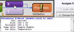
Also, remember that after you load data into a validation control, you can place your mouse pointer on the control to view not only information about the loaded data, but also, different instructions about working with the control. In the figure below, data has been loaded into the X validation control for a PCA analysis.

Viewing information about loaded data

After you have opened the Analysis window and loaded the validation data, you then apply the model to the validation data. To apply the model to the validation data, you can do one of the following:

• On the Analysis window toolbar, click the Calculate/Apply model icon .
• Click the Model control.

Note: Auto-Alignment and Missing Data If the variables in the validation data are not identical to the calibration data variables, you will be informed and asked if Analysis should attempt to perform "Auto-Alignment". For details on this procedure, see Auto-Alignment and Missing Data Replacement.

Clicking the model control to apply the model to validation data

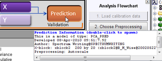
After the model is applied to the validation data, you can place your mouse pointer on the Model control to view information about the model.

Viewing information about the model

Examining and refining the model

After the model is applied, the most relevant plots to create are Scores plots. (Remember, nothing has changed about the Eigenvalues, nothing has changed about the loads and variable statistics - all you have done is apply the model to validation data.)

Note: The examples listed here are not meant to be an exhaustive list of all of the available Plot Controls options for refining a model using a Scores plot. Instead, it is simply to provide representative examples of some of the more commonly used options when applying a model.

1.	On the Analysis window toolbar.click the Plot scores and sample statistics button .

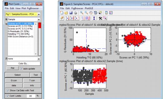
The figure below shows some of the possible Scores plots for when applying the PCA model that you built during the Calibration phase to validation data. Note that initially, the plots show both the calibration data () and the validation data ().

Scores plot showing both calibration data and validation data

2.	Double-click on a plot of interest in the multiplot Figure window to open the plot in its own Figure window, or you can select the plot in the multiplot Figure window, and on the Plot Controls window, click View > Subplots.

3.	With the plot of interest now open in its own Figure window, you can now do one or more of the following to refine the model:

To view only the validation data in the plot, clear the Show Cal Data with Test option in the Plot Controls window. To view the validation data in the context of the calibration data, click the Show Cal Data with Test option again.

Note: You should review a variety of plots with just the validation data, and then with both the validation data and calibration data to ensure that your validation data has the same distribution as your calibration data. For example, plot the Q Residuals versus the T^2 values for the validation data alone, then click the Show Cal Data with Test option to add the calibration data to this plot to confirm that your validation samples cover the same "space" (low Q/low T^2) that your calibration samples cover.

Increase the confidence limits as needed from the default value of 95% to ensure that all of your validation samples are contained within the limits. (Remember, you know the characteristics of your validation data and you know, therefore, that all of the validation data is "good" and must be included in the model.)

Reduce the complexity of the model by choosing a different number of components or factors to retain in the model and then recalculate the model. After you recalculate the model, a new prediction is automatically calculated. (See Changing the number of components for the procedure that describes how to recalculate a model.)

4.	After you are satisfied with the model, save the model.