parafac
Purpose
PARAFAC (PARAllel FACtor analysis) for multi-way arrays
Synopsis
model = parafac(X,initval,options)
pred = parafac(Xnew,model)
options = parafac('options')
Description
PARAFAC will decompose an array of order N (where N
>= 3) into the summation over the outer
product of N vectors (a low-rank model). E.g. if N=3 then the
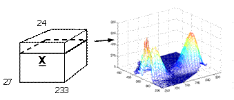
array is size I by J by K. An example of three-way
fluorescence data is shown below..
For example, twenty-seven samples containing different amounts
of dissolved hydroquinone, tryptophan, phenylalanine, and dopa are measured
spectrofluoremetrically using 233 emission wavelengths (250-482 nm) and 24
excitation wavelengths (200-315 nm each 5 nm). A typical sample is also shown.

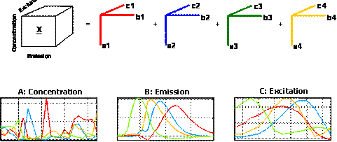
A four-component PARAFAC model of these data will give four
factors, each corresponding to one of the chemical analytes. This is
illustrated graphically below. The first mode scores (loadings in mode 1) in
the matrix A (27×4) contain estimated relative concentrations of the
four analytes in the 27 samples. The second mode loadings B (233×4) are
estimated emission loadings and the third mode loadings C (24×4) are
estimated excitation loadings.

In the PARAFAC algorithm, any missing values must be set to NaN or Inf and are then automatically handled by expectation maximization. This routine
employs an alternating least squares (ALS) algorithm in combination with a line
search. For 3-way data, the initial estimate of the loadings is usually
obtained from the tri-linear decomposition (TLD).
INPUTS:
x = the multiway array to be decomposed, and
ncomp = the number of factors (components) to use, or
model = a PARAFAC model structure (new data are fit to the
model i.e. sample mode scores are calculated).
OPTIONAL INPUTS:
initval = cell array of initial values (initial guess) for
the loadings (e.g. model.loads
from a previous fit). If not used it can be 0 or [], and
options = discussed below.
OUTPUTS:
The output model
is a structure array with the following fields:
modeltype: 'PARAFAC',
datasource: structure
array with information about input data,
date: date
of creation,
time: time
of creation,
info: additional
model information,
loads: 1
by K cell array with model loadings for each mode/dimension,
pred: cell
array with model predictions for each input data block,
tsqs: cell
array with T2 values for each mode,
ssqresiduals: cell
array with sum of squares residuals for each mode,
description: cell
array with text description of model, and
detail: sub-structure
with additional model details and results.
The output pred
is a structure array that contains the approximation of the data if the options
field blockdetails is set to 'all'
(see next).
Options
options = a structure array with the following fields:
display: [
{'on'} | 'off' ], governs level of display,
plots: [ {'final'} | 'all' | 'none' ], governs level of plotting,
weights: [], used for fitting a weighted loss function
(discussed below),
stopcrit: [1e-6
1e-6 10000 3600] defines the stopping criteria as [(relative tolerance)
(absolute tolerance) (maximum number of iterations) (maximum time in seconds)],
init: [ 0 ], defines how parameters are initialized (discussed below),
line: [ 0 | {1}] defines whether to use the line search {default uses
it},
algo: [ {'ALS'} | 'tld' | 'swatld' ] governs algorithm used,
iterative: settings
for iterative reweighted least squares fitting (see help on weights below),
blockdetails: 'standard'
missdat: this option is not yet active,
samplemode: [1], defines which mode
should be considered the sample or object mode,
constraints: {3x1
cell}, defines constraints on parameters (discussed below), and
coreconsist: [ {'on'} | 'off' ], governs
calculation of core consistency (turning off may save time with large data sets
and many components).
The default options can be retrieved using: options = parafac('options');.
WEIGHTS
Through the use of the options field weights it is possible to
fit a PARAFAC model in a weighted least squares sense The input is an array of
the same size as the input data X
holding individual weights for each element. The PARAFAC model is then fit in a
weighted least squares sense. Instead of minimizing the frobenius norm ||x-M||2
where M is the PARAFAC model, the norm ||(x-M).*weights||2 is
minimized. The algorithm used for weighted regression is based on a
majorization step according to Kiers, Psychometrika, 62, 251-266,
1997 which has the advantage of being computationally inexpensive. If
alternatively, the field weights
is set to ‘iterative’
then iteratively reweighted least squares fitting is used. The settings of this
can be modified in the field iterative.cutoff_residuals
which defines the cutoff for large residuals in terms of the number of robust
standard deviations. The lower the number, the more subtle outliers will be
ignored.
INIT
The options field init is used to govern how the initial guess for the
loadings is obtained. If optional input initval is input then options.init is not used.
The following choices for init are available.
Generally, options.init
= 0, will do for well-behaved data whereas options.init = 10, will be suitable for difficult
models. Difficult models are typically those with many components, with very
correlated loadings, or models where there are indications that local minima
are present.
init = 0, PARAFAC chooses initialization {default},
init = 1, uses TLD (unless there are missing values
then random is used),
init = 2, initializes loadings with random values,
init = 3, based on orthogonalization of random values
(preferred over 2),
init = 4, based on singular value decomposition,
init
= 5, based on compression which may be useful for large data, and
init > 5, based on best fit of many (the value options.init) small runs.
CONSTRAINTS
The options field constraints is used to employ constraints on the
parameters. It is a cell array with number of elements equal to the number of
modes of the input data X. Each cell contains a structure array with the
following fields:
nonnegativity: [
{0} | 1 ], a 1 imposes non-negativity.
unimodality: [ {0} | 1 ], a 1
imposes unimodality (1 local maxima).
orthogonal: [ {0} | 1 ], constrain factors
in this mode to be orthogonal.
orthonormal: [
{0} | 1 ], constrain factors in this mode to be orthonormal.
exponential: [
{0} | 1 ], a 1 fits an exponential function to the factors in this mode.
smoothness.weight: [0 to 1], imposes smoothness using
B-splines, values near 1 impose high smoothness and values close to 0, impose
less smoothness.
fixed.position: [
], a matrix containing 1’s and 0’s of the same size as the corresponding
loading matrix, with a 1 indicating where parameters are fixed.
fixed.value: [
], a vector containing the fixed values. Thus, if B is the loading matrix,
then we seek B(find(fixed.position))
= fixed.value. Therefore, fixed.value must be a matrix of the same size
as the loadings matrix and with the corresponding elements to be fixed at their
appropriate values. All other elements of fixed.value are disregarded.
fixed.weight: [
], a scalar (0 <= fixed.weight <= 1) indicating how strongly the fixed.value is imposed. A
value of 0 (zero) does not impose the constraint at all, whereas a value of 1
(one) fixes the constraint.
ridge.weight: [
], a scalar value between 0 and 1 that introduces a ridging in the update
of the loading matrix. It is a penalty on the size of the esimated loadings.
The closer to 1, the higher the ridge. Ridging is useful when a problem is
difficult to fit.
equality.G: [
], matrix with N columns, where N is the number of factors, used with
equality.H. If A
is the loadings for this mode then the constraint is imposed such that GAT
= H. For example, if G is a row vector of ones and H is a
vector of ones (1’s), this would impose closure.
equality.H: [
], matrix of size consistent with the constriant imposed by equality.G.
equality.weight: [
], a scalar (0 <= equality.weight
<= 1) indicating how strongly the equality.H and equality.G is
imposed. A value of 0 (zero) does not impose the constraint at all, whereas a
value of 1 (one) fixes the constraint.
leftprod: [0], If the loading matrix, B is of size JxR,
the leftprod is a matrx G of size JxM. The loading B is then
constrained to be of the form B = GH, where only H is updated.
For example, G may be a certain JxJ subspace, if the loadings are to be
within a certain subspace.
rightprod: [0],
If the loading matrix, B is of size JxR, the rightprod is a matrx G
of size MxR. The loading B is then constrained to be of the form B
= HG, where only H is updated. For example, if rightprod is [1 1 0;0 0 1], then the
first two components in B are forced to be the same.
iterate_to_conv: [0],
Usually the constraints are imposed within an iterative algorithm. Some of the
constraints use iterative algorithms themselves. Setting iterate_to_conv to one, will
force the iterative constraint algorithms to continue until convergence.
timeaxis: [], This field (if supplied) is used as the time axis
when fitting loadings to a function (e.g. see exponential). Therefore, it must have the same
number of elements as one of the loading vectors for this mode.
description: [1x1592
char],
If the constraint in a mode is set as fixed, then the loadings
of that mode will not be updated, hence the initial loadings stay fixed.
Examples
parafac demo
gives a demonstration of the use of the PARAFAC algorithm.
model =
parafac(X,5) fits a five-component PARAFAC model to the array X using default settings.
pred =
parafac(Z,model) fits a parafac model to new data Z. The scores will be taken
to be in the first mode, but you can change this by setting options.samplemodex to the
mode which is the sample mode. Note, that the sample-mode dimension may be
different for the old model and the new data, but all other dimensions must be
the same.
options =
parafac('options'); generates a set of default settings for PARAFAC. options.plots = 0; sets the
plotting off.
options.init
= 3; sets the initialization of PARAFAC to orthogonalized random
numbers.
options.samplemodex
= 2; Defines the second mode to be the sample-mode. Useful, for example,
when fitting an existing model to new data has to provide the scores in the
second mode.
model =
parafac(X,2,options); fits a two-component PARAFAC model with the
settings defined in options.
parafac io
shows the I/O of the algorithm.
See Also
datahat, explode, gram, mpca, outerm, parafac2, preprocess, tld, tucker, unfoldm

